(Picture taken from G-Bot Algorithmic Platform)
Metrics for Algorithmic Trading:
(Tom Gastaldi's)
Direction and Codirection indices [draft version,
please report errors or
suggestions, thanks]
In finance there are several metrics which can be applied to algorithmic trading
as well.
However, a trader may find more useful and intuitive, other, more specific,
dynamic metrics, specifically designed for the context of
automated trading systems and algorithmic trading.
The SDX (Signed Direction Index), SCX (Signed Codirection index) and the other metrics described below have been proposed by Prof. Tom Gastaldi (and also implemented within G-Bot).
Summary of metrics on this page
- $peed
- Sideways %
-
SDX - Signed Direction Index
-
SCX - Signed
Codirection Index
(or "Signed Cointegration Index")
[see
also discussion
linked below]
-
Relative exposure of correlated instruments
Preliminary notes
Algorithmical reference system
The concept of "timeframe" is replaced by a reference system formed by grid lines. This is because an algorithmic trading system, to the purpose of decision taking, focuses mainly on price changes.
Imagine the price range subdivided in intervals
of a given width (based on
a prespecified percentage, for instance 0.1%).
Let's call the
lines marking the intervals, "grid lines" (or "price grid lines"). The distance between 2 given adjacent price grid lines
is called Gridsize and corresponds to a given
price percentage.
The grid line reference system
can be the basis of an algorithmical trading system.
Changing the grid value means expanding or shrinking the
granularity of our computations and might reflect focus on different
"timeframes", except that here our "clock" is defined solely
based on price moves. For instance, the scalps could be defined in terms of
a factor of the gridsize.
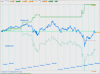
Example (a grid of 0.1%):
(Picture taken from
G-Bot
Algorithmic Platform)
Now we can define some metrics.
$ Speed (of the price) of an instrument
Alternate names: "$peed",
potential exposure
For an algorithmic trader, the concept of volatility (standard deviation of log returns) is somehow useful. However, a more specific concept can be defined, which is even more easily interpretable in an algorithmic trading context, and also can help better managing risk. The concept of "speed" also allows to introduce a "directional" component, which is not present in the volatility concept (volatility is simply the the standard deviation of the log returns).
Definition and algorithm
As the price moves, the grid lines will be "hit" by the price. We consider a dynamic list of "last" hits, where a "hit" is defined as the pair:
Hit = (T, P)
where: T is the instant of the event, and P is the price of the grid line being hit.
A new hit is inserted at the end of the list of hits only if it has a price different from the previous hit. When the length of the list reaches a prespecified size s, the length of the hit list is kept fixed, by removing the oldest entries.
Let's denote the Hit list as:
Hit(0) , .... , Hit(s-1)
Within this list, we consider k (k <=
s) terms equispaced (thus possibly resampling the
list to size k):
Hit(0) , .... , Hit(k-1)
We define (k-1) price changes, and (k-1) elapsed time intervals, defined as follows:
ΔP(i) = P(i) - P(i-1) i = 1, ... , k-1
ΔT(i) = T(i) - T(i-1) i = 1, ... , k-1
the $peed is defined as follows ("absolute" version):
Σ | ΔP(i) |
$peed = ----------------- *
ContractMultiplier * UserPacketSize
Σ ΔT(i)
where
UserPacketSize denotes the reference order size used by the trader (say the
tipical order size he intends to use as reference size for exposure evaluation.
The
UserPacketSize can also be a dynamic quantity: for
instance recalibrated realtime by the trading algorithm).
It is also possible, and
indeed more useful, to consider a variant which would not depend on the packet
size of each instrument in the folio. This could be called "intrinsic $peed" and
in a similar way as, but replacing UserPacketSize with a
constant, fixed for all instrumens of a given type (for instance, 100 for STK,
CFD, 1 for FUT, FOP, OPT, 10K for CASH).
This would allow for instance to correctly use a correlated instrument to hedge another instrument. In fact, for precise hedging, we need to take into account both the
notional amount invested, but also the "$peeds" at which the two different
instruments move.
It also makes sense to consider a "signed" version, where the
ΔP(i) are considered with their respective signs.
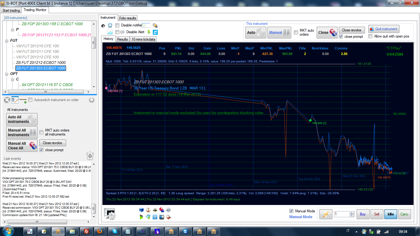
Example:
($peeds of various instruments (futures): picture taken from
G-Bot
Algorithmic Platform: this picture
denotes a badly unbalanced folio, where 2 instruments are towering over the
folio)
Sideways percentage of speed, horizontal component of
speed
When an instrument moves at a certain speed, its "trajectory" can develop mostly
sideways, or it can be "trending" up or down. This percentage index expresses how
much of the total speed of the instrument is expressed sideways. Clearly, the
complement to 100 is the percentage of the speed expressed directionally.
Definition and algorithm
We decompose the total speed into 2 components: a sideways component and a directional component. Alternatively, we can say, an "horizontal" component and "vertical" component.
Speed = Sydeways Speed + Vertical Speed
where:
Vertical Speed = V * Speed
Sideways Speed = S * Speed
with S + V = 1
The vertical-component coefficient V is defined as:
|
Σ ( for ΔP(i) > 0) | ΔP(i) | - Σ ( for ΔP(i) < 0)
| ΔP(i) | |
V = ----------------------------------------------------------------
Σ | ΔP(i) |
Given the vertical speed, we can obtain the horizontal speed by difference: Horizontal Speed = Speed - Vertical Speed
Finally, the Trending and Sideways percentages are defined as:
Vertical Speed
Trending % = ----------------------- *
100 = V * 100
Speed
Horizontal Speed
Sideways % = ----------------------- *
100
= ( 1 - V ) * 100 = S * 100
Speed
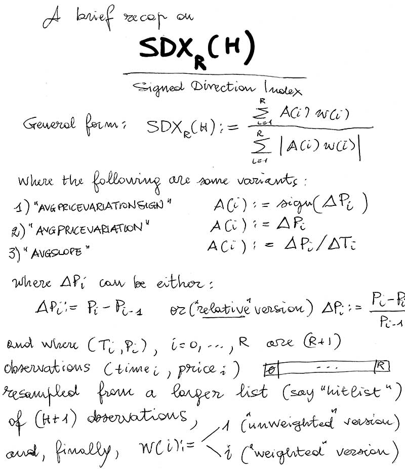
SDX - Signed Direction Index (of the price) of an instrument
The V coefficient of the directional component, taken with sign (and multiplied by 100) provides a "local" assessment of direction and "momentum" of the price of an instrument:
Σ (for ΔP(i) > 0) | ΔP(i) | - Σ (for ΔP(i) < 0)
| ΔP(i) |
SDX = =
------------------------------------------------------------- * 100
Σ | ΔP(i) |
it ranges between -100 (downward move) and 100 (upward move). Values (positive or negative) near 0, indicate a condition of "sideways" market.
It should be noted that the above sums do not run over all hits, but they must be
taken on a subsample of equispaced points within the hit list. The number of
intervals considered are a parameter of the SDX (and it's advisable they be an
even number, to allow SDX to be equal to 0). Thus, the SDX would be computed by
taking a given number of points equispaced within the hit list.
I usually use the notation SDXR(H), where R denotes the number of differences in
the resampled list, and H the same in the original list.
One can compute a Short term SDX and
a Long term SDX, depending on the
"priceframe" or hit list length
H considered. This is also used by G-Bot for some "entry styles" [good choices of hit list lengths for SDX_Lt and
SDX_St, are, for instance H=21
for a 100% volatility and scaled according to volatility (but never
less then the resampling size, obviously), while for the long
term, we multiply for a given factor (for instance 4, 5) and H=100, while, for
instance, R=5].
Note that SDX definition can stand alone and does not depend on
defining the $peed. Actually $peed could take alternate definitions (like
variants defined by the user) without affecting the definition of the SDX.
Also note that in actual implementation, we need not to refer to actual "hits"
of gridlines, but it is sufficient that the price moves away from the last
recorded price of a prespecified amount (for instance, the 0.1%)
Another variant, which I prefer, can be obtained by considering also the time
necessary for each price variation, as follows:
Σ ( P(i) - P(i-1) ) / ( T(i) - T(i-1) )
Σ ΔP(i) / ΔT(i)
SDXR(H) =
---------------------------------------- * 100 =
------------------- * 100
Σ | P(i) - P(i-1) |
/ ( T(i) - T(i-1) ) Σ | ΔP(i) |
/ ΔT(i)
which can be intuitively interpreted as a normalized average of "slopes".
Weighted version
A weighted version can also be considered, by assigning different (positive) weights w(i) to the consecutive price changes ΔP(i)
Σ
w(i) ΔP(i) / ΔT(i)
SDXR(H) = --------------------------- *
100
Σ |
w(i) ΔP(i) |
/ ΔT(i)
Note. It is important to remark that, in our approach (reflected in the G-BOT project), we do not make any "predictive" use of the SDX. The SDX is instead used merely to provide "check points" for internal "coherence" of the player cloud, and make sure that the preserved past trading information is used in the best possible way, to the purpose of hedging, and eventually have the algo "converge" to a permanent sell / buy avg "crossover".
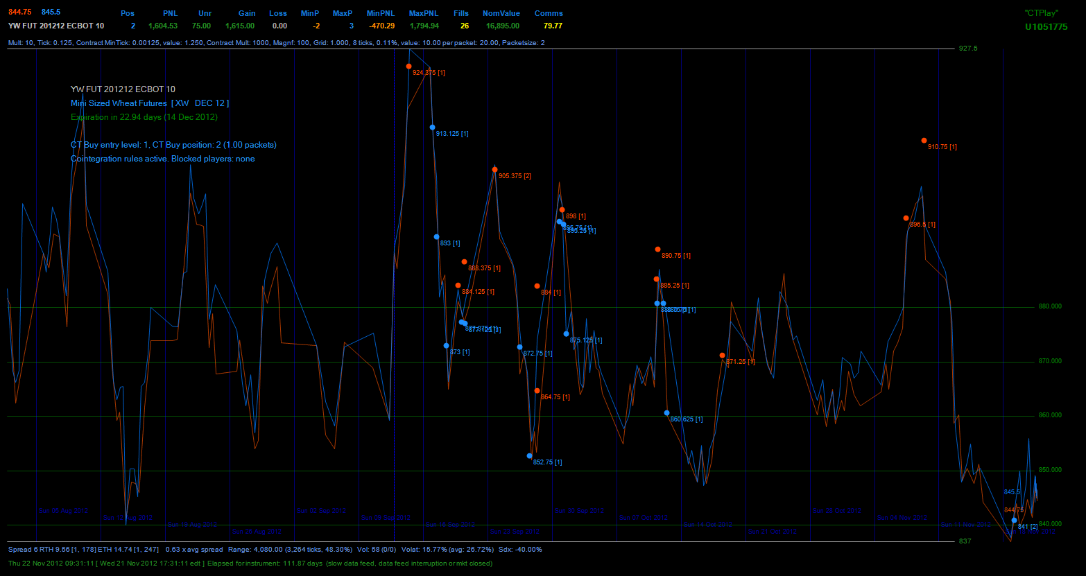
Example
This is an example of scalping carried out by using the SDX. This is a picture
of actual trading with real money, sent to me by a fund manager, along with the
following message:
"Here is a great example of G-bot at work. Simply put it
has traded like a maestro. There are many other examples of similar trading
patterns on other instruments.
Tom are you sure you don’t have sight of the future ?
J." [ Wed, Nov 21,
2012 at 11:33 PM ]
Relationships between the above concepts
From the definitions, one may notice that :
Trending % = | SDX |
Sideways % = 100 - | SDX |
As it is intuitive, the trending percentage is given by the absolute value of the signed direction index.
It is also possible to create metrics based on the "divergence" of 2 SDXs (one "short-term" and one "longer-term").
One fundamental (and rather persistent and often structural) aspect in the market, which is immediately evident when trading large folios, is the fact that some instruments "track each other" ("positively" or "negatively"). This can result in price curves which "look" essentially the same (example DIG and ERX) or that are essentially "specular" (e.g., DIG and DUG).
Sometimes we hear talking about positive or negative "correlation"
or "cointegration" between
instruments.
In statistics, the "correlation coefficient" is a measure of
"linear" correlation.
Here I introduce a simple index to measure the tendency of two price curves to
look like the same (index = 1) or to be a mirror image of each other (index = -1).
Denote these 2 lists (the recording times are the same for the two lists) as:
P1(0), P1(1), ... , P1(k-1), (for Instrument 1)
P2(0), P2(1), ... , P2(k-1), (for Instrument 2)
A simple, but effective, cointegration index, ranging in the interval [-1, 1] can be obtained (on a resampled set of points) as:
Σ
( sgn (
ΔP1(i) ) * sgn (
ΔP2(i) ) )
SCX =
-----------------------------------
N
where sgn() is the sign operator, N is number of the products considered in the above sum (possibly k-1), and the sum is taken over the nonnull products (factors
equal to zero, that in practice
would be rare and irrelevant, could be possibly: considered, skipped, or the result of product
defined according to a convenient convention).
Note that, just as for the computation of SDX, we operate on a
resampled set. (For instance, one might take a maximum of 100 differences). This is important to keep the
computation consistent, whatever is the number of prices collected for the computations,
and would allow to make possible comparisons.
This index will range between -1 and 1. A value of 1 means perfect
"codirection" (they "track each other"); -1 is also a perfect (negative)
codirection. Values near 0 will indicate situations where the 2 instruments
are, say, in no
codirection relation:
-1 ("specular" shapes) -------- 0 (no cointegration) --------- 1 (similar
shapes)
Another useful version, which also takes into account the size of price
variations and time intervals, is the following:
Σ
(
ΔP1(i) /T(i) *
ΔP2(i)/T(i) )
SCX =
-----------------------------------
Σ |
ΔP1(i)/T(i) *
ΔP2(i)/T(i) |
where T(i) denotes the time interval between two consecutive prices (intuitively, a mixed moment of slopes).
In practice, (independent) random instruments will
have small | SCX |. Absolute values depend on the resampling size steps one
uses. For instance with 100 steps, values less than 0.3 are in the realm of no
strong codirection yet. Larger absolute values (0.6 to 1) denote good "codirection". Around and beyond 0.9 we
have a practical coincidence of price curves (or perfect specular shape, in case
of negative correlation).
This index will not limit itself to capture a linear component of the
relationship (as it happens for classical cointegration indices), but it is
sensitive to any form of relationship. This is particularly appropriate
as the concept of linearity is just an elementary mental abstraction that finds no place in
the real market.
This is also the reason why we might prefer to
call it a "codirection index" in order to signify its broader scope.
See also this public discussion on Linkedin for more insight:
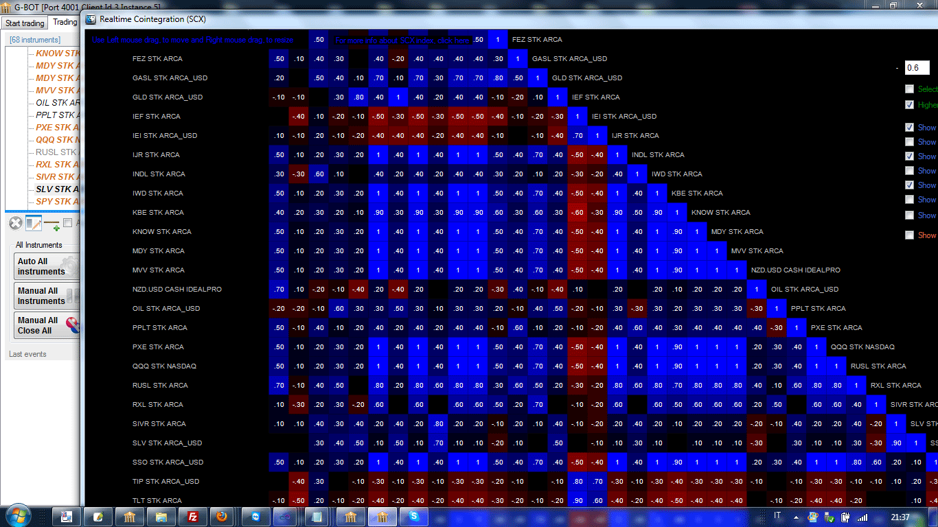
Example. SCX for various pairs of instruments (SCX matrix)
For this index too, one might consider an obvious "weighted" version.
Another possible application of this index, in addition to hedging functionalities, is within
arbitrage algorithms which would exploit the relative
"disalignment" of the involved instruments.
(Clearly, in such a case, we will also need to appropriately determine the
relative direction of each instrument w.r.t. the other one, which is pretty
straightforward to do.)
The main application is, however, in folio trading, where the SCX can be
effectively used to turn dependences into a powerful hedging tool. In fact,
exposure of some instruments can obviously be appropriately hedged by the exposure of other strongly
cointegrated (large absolute value of SCX ) instruments.
Exposure of a correlated set of
instrument, relative to an instrument in a folio
Define for each instrument , say I, in a folio of instruments the
following quantities:
SAE := "Signed (Volatility-Adjusted) Exposure"
REC := "Relative Exposure of Correlated Instruments"
Such quantities are defined as follows:
SAE := Closing Price * Position with sign * Multiplier * Volatility * 0.001 (so with $K as unit
of measure)
for instance, an instrument could have an exposure of 15.56K, and so on.
While, the "Relative Exposure of Correlated Instruments" is defined as follows:

Where corr(I,J) indicates your preferred correlation (or "codirection") metrics, such as for instance the SCX
This quantity, along with the instrument exposure SEA(I) is useful to rebalance exposure across layers, for instance, according to the following scheme:

The meaning of the schema seems intuitive. Let's consider, for
instance, SAE(I) > 0 and REC(I) > 0. In this case, both the instrument I and the
set of correlated instruments C(I) have a positive exposure. So a SELL order of
I would have an "hedging" effect on the exposure. Let's consider for instance
SAE(I) < 0 and REC(I) > 0. In this case, I is negatively exposed (it has a short
position), while the correlated instruments are "contrasting" this exposure
(either through opposite position under positive correlation or same side
position under negative correlation). Now, depending on which of the 2 exposure
is larger (REC(I) or SAE(I)), we have an exposure reduction either by Selling of
Buying (respectively) I. The other 2 cases are analogous.
Similarly, they offer an indication of the "role" of I within the folio. For
instance, if SAE(I) > 0 and REC(I) < 0 and |SAE(I)| < |REC(I)| we can interpret
the instrument I as having an "hedging value" within the folio and that it's
suitable for (signed) position increase. The interpretations of the other cases,
can be done applying a similar logic.